43 excel 2013 pie chart labels

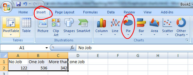
Add a Data Callout Label to Charts in Excel 2013 In the upper right corner, next to your chart, click the Chart Elements button (plus sign), and then click Data Labels. A right pointing arrow will appear, click on this arrow to view the submenu. Select Data Callout. Once the Data Callout Labels have been added, you can re-position them by clicking on their borders and dragging to a new position. How to Make a Pie Chart in Excel 2013 - Solve Your Tech How to Make Excel 2013 Pie Charts Open your spreadsheet. Select the data. Click the Insert tab. Select the Pie Chart button. Choose the desired pie chart style. Our article continues below with additional information on making a piechart in Excel, including pictures of these steps. How to Create a Pie Chart in Excel (Guide with Pictures)

Vary the colors of same-series data markers in a chart In the Format Data Series pane, click the Fill & Line tab, expand Fill, and then do one of the following: To vary the colors of data markers in a single-series chart, select the Vary colors by point check box. To display all data points of a data series in the same color on a pie chart or donut chart, clear the Vary colors by slice check box.

Excel 2013 pie chart labels

How to Create and Label a Pie Chart in Excel 2013 Click on the pie chart that appeared on your screen, and then, out of the 3 boxes that will appear on its right side, click on the cross. Ask Question Step 8: Label the Chart Check the "Data Labels" square and the labels will appear on the pie chart. Congratulations, you have successfully created a labeled pie chart. How can I control the color of individual pie chart segments in Excel? I would like to be able to control the color of the sections in a pie chart programmically. Ideally my chart would be based on a 3-column table with the columns being: The Data Value, The Label, and the Pie Chart Color Value. The color values would be that same numbers one sees in Access form properties. Thanks, Steve How to Create and Format a Pie Chart in Excel - Lifewire To add data labels to a pie chart: Select the plot area of the pie chart. Right-click the chart. Select Add Data Labels . Select Add Data Labels. In this example, the sales for each cookie is added to the slices of the pie chart. Change Colors

Excel 2013 pie chart labels. Microsoft Excel Tutorials: Add Data Labels to a Pie Chart To add the numbers from our E column (the viewing figures), left click on the pie chart itself to select it: The chart is selected when you can see all those blue circles surrounding it. Now right click the chart. You should get the following menu: From the menu, select Add Data Labels. New data labels will then appear on your chart: Group Smaller Slices in Pie Charts to Improve Readability Select "Pie of Pie" chart, the one that looks like this: At this point the chart should look something like this: 2. Click on any slice and go to "format series". Click on any slice and hit CTRL+1 or right click and select format option. In the resulting dialog, you can change the way excel splits 2 pies. We will ask excel to split the ... How to Add and Format Text Boxes in a Chart in Excel 2013 To add a text box in Excel 2013 like the one shown to the chart when a chart is selected, select the Format tab under the Chart Tools contextual tab. Then, click the Insert Shapes drop-down button to open its palette where you select the Text Box button. To insert a text box in a worksheet when a chart or some other type of graphic isn't ... How to Create Pie Charts in Excel (In Easy Steps) Click the + button on the right side of the chart and click the check box next to Data Labels. 10. Click the paintbrush icon on the right side of the chart and change the color scheme of the pie chart. Result: 11. Right click the pie chart and click Format Data Labels. 12. Check Category Name, uncheck Value, check Percentage and click Center.

Microsoft Excel Tutorials: How to Format Pie Chart segments Move a Pie Chart Segement in Excel. To move the slice that you've just coloured, click back on Series Options from the options on the left: Now click the Close button. Your chart should look something like this one: Change the rest of the slices in exactly the same way. You can format the rest of the chart exactly like you did for the Bar chart. Excel 2013 Pie Chart Category Data Labels keep Disappearing GeneLandriau2 Created on April 19, 2016 Excel 2013 Pie Chart Category Data Labels keep Disappearing Hi All, I have a table in Excel 2013 with 2 slicers - Region and Product Hierarachy, with 5 values in each. I've built a couple pie charts that update when you click on the slicers, to show Market Share by Market Segment. How to Create Charts From the Ribbon in Excel 2013 - dummies Insert Pie or Doughnut Chart to preview your data as a 2-D or 3-D pie chart or 2-D doughnut chart Insert Scatter (X,Y) or Bubble Chart to preview your data as a 2-D scatter (X,Y) or bubble chart When using the galleries attached to these chart command buttons on the Insert tab to preview your data as a particular chart style, you can embed the ... Pie Charts in Power View - YouTube Pie charts are simple or sophisticated in Power View. This video shows you how to create a basic pie chart, add slices, and drill down and drill up.Olympics ...

How to modify Chart legends in Excel 2013 - Stack Overflow The words in the legend are sourced from the series name. You can point the series name to any cell in the spreadsheet. In the screenshot, the original series names were one, two and three. In the series definition, they got re-pointed to the cells that say blue, red and green. Depending on your data and requirements this can be made dynamic. Share Rotate a pie chart - support.microsoft.com Right-click any slice of the pie chart > Format Data Series. In the Format Data Point pane in the Angle of first slice box, replace 0 with 120 and press Enter. Now, the pie chart looks like this: If you want to rotate another type of chart, such as a bar or column chart, you simply change the chart type to the style that you want. Display data point labels outside a pie chart in a paginated report ... Create a pie chart and display the data labels. Open the Properties pane. On the design surface, click on the pie itself to display the Category properties in the Properties pane. Expand the CustomAttributes node. A list of attributes for the pie chart is displayed. Set the PieLabelStyle property to Outside. Set the PieLineColor property to Black. How to create pie of pie or bar of pie chart in Excel? The following steps can help you to create a pie of pie or bar of pie chart: 1. Create the data that you want to use as follows: 2. Then select the data range, in this example, highlight cell A2:B9. And then click Insert > Pie > Pie of Pie or Bar of Pie, see screenshot: 3. And you will get the following chart: 4.

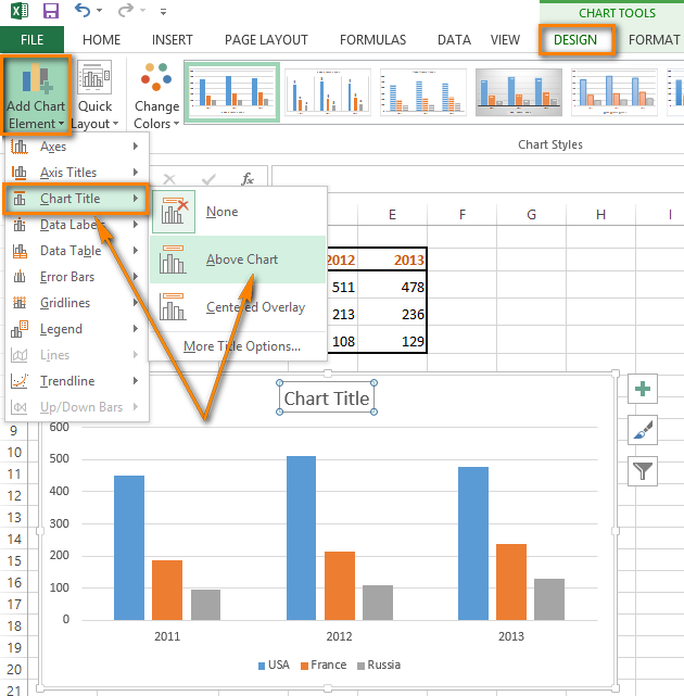
How to add titles to charts in Excel 2016 - 2010 in a minute.

Excel 2013 Chart label not displaying The pie chart displays the wedge within the chart itself, but does not display the label. At the moment I have data labels with percentages. All other labels display, of which there are 7. I found a solution that fixes the problem each time it arises and that is to select Chart Tools/Format/Series 1 data labels and then Format Selection.

How to Create Multi-Category Chart in Excel - Excel Board

Microsoft Excel 2013 - How to increase gap between slices in Pie Chart ... Step 1. Open the excel sheet where the Pie Chart graph is added; in Microsoft Excel 2013 application. Step 2. Select the Pie Chart. Excel application will display "Series Options" properties in the "Format Data Series" pane. Microsoft Excel 2013 - Pie Chart - Series Options Step 3.

Stats - Pie Charts

Pie Chart Rounding in Excel - Peltier Tech Both charts below use the same data range, three cells each containing the value 1. Each pie wedge is 1/3 of the total, 33.333333…%, rounded to 33%. However, the first chart reports percentages of 34%, 33%, and 33%. The second chart, with one added decimal digit of precision, correctly displays 33.3% for all three wedges.

How to add titles to charts in Excel 2010 / 2013 in a minute.

Excel Chart VBA - 33 Examples For Mastering Charts in Excel VBA Charts.Add End Sub 3. Adding New Chart for Selected Data using Charts.Add Method : In Existing Sheet using Excel VBA We can use the Charts.Add method to create a chart in existing worksheet. We can specify the position and location as shown below. This will create a new chart in a specific worksheet.

Share :