38 how to add specific data labels in excel

Custom Data Labels with Colors and Symbols in Excel Charts - [How To] Step 4: Select the data in column C and hit Ctrl+1 to invoke format cell dialogue box. From left click custom and have your cursor in the type field and follow these steps: Press and Hold ALT key on the keyboard and on the Numpad hit 3 and 0 keys. Let go the ALT key and you will see that upward arrow is inserted. Excel tutorial: How to use data labels Generally, the easiest way to show data labels to use the chart elements menu. When you check the box, you'll see data labels appear in the chart. If you have more than one data series, you can select a series first, then turn on data labels for that series only. You can even select a single bar, and show just one data label.

excel - Add Data Labels with VBA - Stack Overflow 3 Answers. Sorted by: 1. The issue is that. If Sheet1.Range ("W11") = "TRUE". is not true. If you Debug.Print Sheet1.Range ("W11") = "TRUE" it will return false instead of the expected true. The cause is that Sheet1.Range ("W11") returns a boolean not a string in this case. You can verify the return type with.

How to add specific data labels in excel

How to add and customize chart data labels - Get Digital Help Double press with left mouse button on with left mouse button on a data label series to open the settings pane. Go to tab "Label Options" see image to the right. This setting allows you to change the number formatting of the data labels. The image below shows numbers formatted as dates. Add a DATA LABEL to ONE POINT on a chart in Excel Steps shown in the video above: Click on the chart line to add the data point to. All the data points will be highlighted. Click again on the single point that you want to add a data label to. Right-click and select ' Add data label ' This is the key step! Right-click again on the data point itself (not the label) and select ' Format data label '. How to Use Cell Values for Excel Chart Labels Select the chart, choose the "Chart Elements" option, click the "Data Labels" arrow, and then "More Options." Uncheck the "Value" box and check the "Value From Cells" box. Select cells C2:C6 to use for the data label range and then click the "OK" button. The values from these cells are now used for the chart data labels.

How to add specific data labels in excel. How to Change Excel Chart Data Labels to Custom Values? First add data labels to the chart (Layout Ribbon > Data Labels) Define the new data label values in a bunch of cells, like this: Now, click on any data label. This will select "all" data labels. Now click once again. At this point excel will select only one data label. Add or remove data labels in a chart - support.microsoft.com To label one data point, after clicking the series, click that data point. In the upper right corner, next to the chart, click Add Chart Element > Data Labels. To change the location, click the arrow, and choose an option. If you want to show your data label inside a text bubble shape, click Data Callout. How to add or move data labels in Excel chart? - ExtendOffice 2. Then click the Chart Elements, and check Data Labels, then you can click the arrow to choose an option about the data labels in the sub menu. See screenshot: In Excel 2010 or 2007. 1. click on the chart to show the Layout tab in the Chart Tools group. See screenshot: 2. Then click Data Labels, and select one type of data labels as you need ... How to create Custom Data Labels in Excel Charts Add default data labels Click on each unwanted label (using slow double click) and delete it Select each item where you want the custom label one at a time Press F2 to move focus to the Formula editing box Type the equal to sign Now click on the cell which contains the appropriate label Press ENTER That's it.

How to add data labels from different column in an Excel chart? Right click the data series in the chart, and select Add Data Labels > Add Data Labels from the context menu to add data labels. 2. Click any data label to select all data labels, and then click the specified data label to select it only in the chart. 3. Adding rich data labels to charts in Excel 2013 - Microsoft 365 Blog Putting a data label into a shape can add another type of visual emphasis. To add a data label in a shape, select the data point of interest, then right-click it to pull up the context menu. Click Add Data Label, then click Add Data Callout . The result is that your data label will appear in a graphical callout. Apply Custom Data Labels to Charted Points - Peltier Tech Click again on a label to select just that specific label. Double click on the label to highlight the text of the label, or just click once to insert the cursor into the existing text. Type the text you want to display in the label, and press the Enter key. Repeat for all of your custom data labels. How to find, highlight and label a data point in Excel scatter plot Select the Data Labels box and choose where to position the label. By default, Excel shows one numeric value for the label, y value in our case. To display both x and y values, right-click the label, click Format Data Labels…, select the X Value and Y value boxes, and set the Separator of your choosing: Label the data point by name

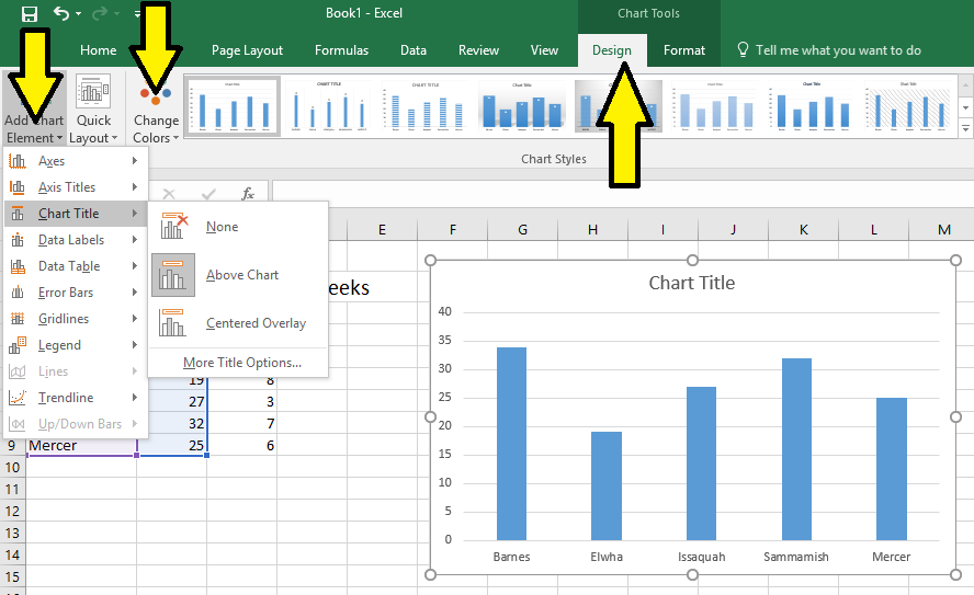
How to Print Labels from Excel - Lifewire Select Mailings > Write & Insert Fields > Update Labels . Once you have the Excel spreadsheet and the Word document set up, you can merge the information and print your labels. Click Finish & Merge in the Finish group on the Mailings tab. Click Edit Individual Documents to preview how your printed labels will appear. Select All > OK . How to Add Labels to Scatterplot Points in Excel - Statology Step 3: Add Labels to Points Next, click anywhere on the chart until a green plus (+) sign appears in the top right corner. Then click Data Labels, then click More Options… In the Format Data Labels window that appears on the right of the screen, uncheck the box next to Y Value and check the box next to Value From Cells. Add Custom Labels to x-y Scatter plot in Excel Step 1: Select the Data, INSERT -> Recommended Charts -> Scatter chart (3 rd chart will be scatter chart) Let the plotted scatter chart be. Step 2: Click the + symbol and add data labels by clicking it as shown below. Step 3: Now we need to add the flavor names to the label. Now right click on the label and click format data labels. Excel charts: add title, customize chart axis, legend and data labels ... Depending on where you want to focus your users' attention, you can add labels to one data series, all the series, or individual data points. Click the data series you want to label. To add a label to one data point, click that data point after selecting the series. Click the Chart Elements button, and select the Data Labels option.

5 Minitab graphs tricks you probably didn’t know about - Master Data Analysis

Improve your X Y Scatter Chart with custom data labels Go to tab "Insert". Press with left mouse button on the "scatter" button. Press with right mouse button on on a chart dot and press with left mouse button on on "Add Data Labels". Press with right mouse button on on any dot again and press with left mouse button on "Format Data Labels". A new window appears to the right, deselect X and Y Value.

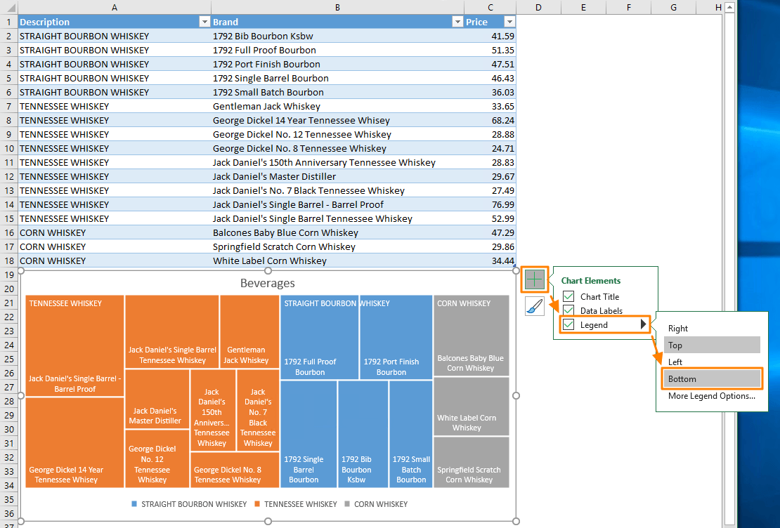
Treemap Excel Charts: The Perfect Tool for Displaying Hierarchical Data

Custom Chart Data Labels In Excel With Formulas Follow the steps below to create the custom data labels. Select the chart label you want to change. In the formula-bar hit = (equals), select the cell reference containing your chart label's data. In this case, the first label is in cell E2. Finally, repeat for all your chart laebls.

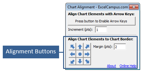
Move and Align Chart Titles, Labels, Legends with the Arrow Keys - Excel Campus

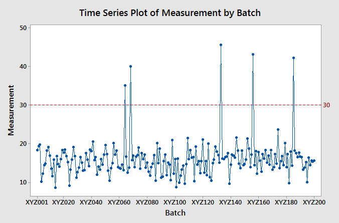
Excel, giving data labels to only the top/bottom X% values 1) Create a data set next to your original series column with only the values you want labels for (again, this can be formula driven to only select the top / bottom n values). See column D below. 2) Add this data series to the chart and show the data labels. 3) Set the line color to No Line, so that it does not appear! 4) Volia! See Below! Share

How Can You Calculate Correlation Using Excel? | Investopedia

How to Add Data Labels to an Excel 2010 Chart - dummies Select where you want the data label to be placed. Data labels added to a chart with a placement of Outside End. On the Chart Tools Layout tab, click Data Labels→More Data Label Options. The Format Data Labels dialog box appears.

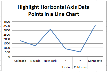
How-to Highlight Specific Horizontal Axis Labels in Excel Line Charts

How to Customize Your Excel Pivot Chart Data Labels - dummies The Data Labels command on the Design tab's Add Chart Element menu in Excel allows you to label data markers with values from your pivot table. When you click the command button, Excel displays a menu with commands corresponding to locations for the data labels: None, Center, Left, Right, Above, and Below. None signifies that no data labels ...

Graphing with Excel - BIOLOGY FOR LIFE

Add Data Labels to Specific Points - MrExcel Message Board Platform Windows Sep 20, 2015 #2 you can click the point a couple of time and then tell it what to display, label or value, if that dosen't work you can always use a text box You must log in or register to reply here. Excel contains over 450 functions, with more added every year. That's a huge number, so where should you start?

Breaking down hierarchical data with Treemap and Sunburst charts | Microsoft 365 Blog

Format Data Labels in Excel- Instructions - TeachUcomp, Inc. To do this, click the "Format" tab within the "Chart Tools" contextual tab in the Ribbon. Then select the data labels to format from the "Chart Elements" drop-down in the "Current Selection" button group. Then click the "Format Selection" button that appears below the drop-down menu in the same area.

Charting Survey Results in Excel - Xelplus - Leila Gharani

Add data labels and callouts to charts in Excel 365 - EasyTweaks.com The steps that I will share in this guide apply to Excel 2021 / 2019 / 2016. Step #1: After generating the chart in Excel, right-click anywhere within the chart and select Add labels . Note that you can also select the very handy option of Adding data Callouts.

Share :