41 excel column chart labels
Change axis labels in a chart in Office - support.microsoft.com The chart uses text from your source data for axis labels. To change the label, you can change the text in the source data. If you don't want to change the text of the source data, you can create label text just for the chart you're working on. In addition to changing the text of labels, you can also change their appearance by adjusting formats. How to add or move data labels in Excel chart? - ExtendOffice In Excel 2013 or 2016. 1. Click the chart to show the Chart Elements button . 2. Then click the Chart Elements, and check Data Labels, then you can click the arrow to choose an option about the data labels in the sub menu. See screenshot: In Excel 2010 or 2007. 1. click on the chart to show the Layout tab in the Chart Tools group. See ...
How to group (two-level) axis labels in a chart in Excel? Select the source data, and then click the Insert Column Chart (or Column) > Column on the Insert tab. Now the new created column chart has a two-level X axis, and in the X axis date labels are grouped by fruits. See below screen shot: Group (two-level) axis labels with Pivot Chart in Excel

Excel column chart labels
Excel tutorial: How to customize axis labels Instead you'll need to open up the Select Data window. Here you'll see the horizontal axis labels listed on the right. Click the edit button to access the label range. It's not obvious, but you can type arbitrary labels separated with commas in this field. So I can just enter A through F. When I click OK, the chart is updated. Excel charts: add title, customize chart axis, legend and data labels Click anywhere within your Excel chart, then click the Chart Elements button and check the Axis Titles box. If you want to display the title only for one axis, either horizontal or vertical, click the arrow next to Axis Titles and clear one of the boxes: Click the axis title box on the chart, and type the text. How to Add Labels to Show Totals in Stacked Column Charts in Excel The chart should look like this: 8. In the chart, right-click the "Total" series and then, on the shortcut menu, select Add Data Labels. 9. Next, select the labels and then, in the Format Data Labels pane, under Label Options, set the Label Position to Above. 10. While the labels are still selected set their font to Bold. 11.
Excel column chart labels. Create a multi-level category chart in Excel - ExtendOffice Select the dots, click the Chart Elements button, and then check the Data Labels box. 23. Right click the data labels and select Format Data Labels from the right-clicking menu. 24. In the Format Data Labels pane, please do as follows. 24.1) Check the Value From Cells box; Excel pie chart labels overlap With many data labels , the task becomes quickly boring and time-consuming. But wait, there is a third option using a duplicate series on a secondary axis. Excel . Details: Overlap Pie Charts In Excel . Excel . Details: STEP 1: Select all the cells in the table. STEP 2: Go to Insert Tab > In the Charts Group, click on the Clustered Column Chart ... Adding Labels to Column Charts | Online Excel Training | Kubicle To add data labels, just right-click on a data series and click add data labels. To see the data labels clearly, I'll need to select them and change their color to white. The data labels are determined by the vertical axis of your chart. Currently, the vertical axis shows millions, therefore, my data labels are shown in millions as well. How to Insert Axis Labels In An Excel Chart | Excelchat Figure 2 - Adding Excel axis labels. Next, we will click on the chart to turn on the Chart Design tab. We will go to Chart Design and select Add Chart Element. Figure 3 - How to label axes in Excel. In the drop-down menu, we will click on Axis Titles, and subsequently, select Primary Horizontal. Figure 4 - How to add excel horizontal axis ...
How to Create a Bar Chart With Labels Above Bars in Excel In the Format Data Labels pane, under Label Options selected, set the Label Position to Inside End. 16. Next, while the labels are still selected, click on Text Options, and then click on the Textbox icon. 17. Uncheck the Wrap text in shape option and set all the Margins to zero. The chart should look like this: 18. Data Labels in Excel Pivot Chart (Detailed Analysis) 7 Suitable Examples with Data Labels in Excel Pivot Chart Considering All Factors 1. Adding Data Labels in Pivot Chart 2. Set Cell Values as Data Labels 3. Showing Percentages as Data Labels 4. Changing Appearance of Pivot Chart Labels 5. Changing Background of Data Labels 6. Dynamic Pivot Chart Data Labels with Slicers 7. Change the format of data labels in a chart To get there, after adding your data labels, select the data label to format, and then click Chart Elements > Data Labels > More Options. To go to the appropriate area, click one of the four icons ( Fill & Line, Effects, Size & Properties ( Layout & Properties in Outlook or Word), or Label Options) shown here. How to I rotate data labels on a column chart so that they are ... To change the text direction, first of all, please double click on the data label and make sure the data are selected (with a box surrounded like following image). Then on your right panel, the Format Data Labels panel should be opened. Go to Text Options > Text Box > Text direction > Rotate
How to Change Font Size of Data Labels in Excel - ExcelDemy Fourthly, select the whole graph and click on the Chart Elements option and go to the Data Labels. After that, you will get the result like the below image. Next, select the data chart and go to the Home tab. Then, choose the font size accordingly. Finally, the following result will come up on your screen. 2. how to align x-axis labels in column chart? - MrExcel Message Board The Excel help page "Change the display of chart axes" ( click here) [1] explains: "You can also change the horizontal alignment of axis labels, by right-clicking the axis, and then click Align Left Button image, Center Button image, or Align Right Button image on the Mini toolbar." When I do that with labels at -45 deg as above, I see very ... Column Chart in Excel (In Easy Steps) Column charts are used to compare values across categories by using vertical bars. To create a column chart, execute the following steps. 1. Select the range A1:A7, hold down CTRL, and select the range C1:D7. 2. On the Insert tab, in the Charts group, click the Column symbol. 3. Click Clustered Column. Note: only if you have numeric labels ... How to Directly Label Stacked Column Charts in Excel On the worksheet, right-click the chart and then, on the shortcut menu, click Select Data. 4. Next, In the Select Data Source dialog box, click on the Add button under Legend Entries (Series). 5. In the Edit Series dialog box, type "Labels" in the Series name edit box and refer to cell B13 in the Series values edit box as per the below screenshot:
Add Total To Stacked Bar Chart Excel - Chart Walls
Stagger long axis labels and make one label stand out in an Excel ... Select any column and press Ctrl+1 to open the Format Data Series task pane. In the Series Options, set the Series Overlap to 100%. You can also set the Gap Width to 50% to give the columns more presence on the chart. Use the "+" chart skittle to remove the legend and gridlines. Add a chart title if desired. The chart will now look like this.
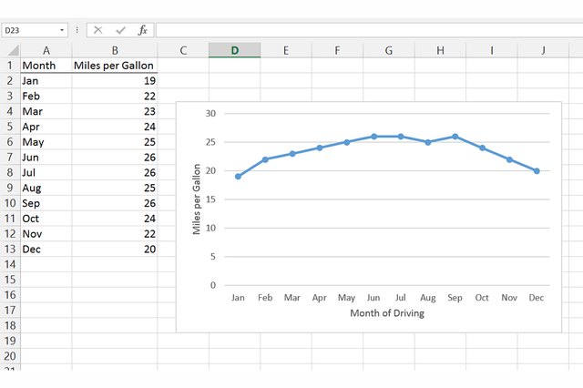
Excel - Line Chart
Chart label in round figures | MrExcel Message Board Apr 29, 2018. #2. If you have chosen the "Add Values From Cell" feature then the format should follow that of the linked cells so you can just format those the way you want or you can select the labels and edit the number format in the chart formatting wizard. in any case, you do not need to label each data point in your series, try to label ...
How to Add an Axis Title to an Excel Chart | Techwalla.com
Add or remove data labels in a chart - support.microsoft.com Click the data series or chart. To label one data point, after clicking the series, click that data point. In the upper right corner, next to the chart, click Add Chart Element > Data Labels. To change the location, click the arrow, and choose an option. If you want to show your data label inside a text bubble shape, click Data Callout.
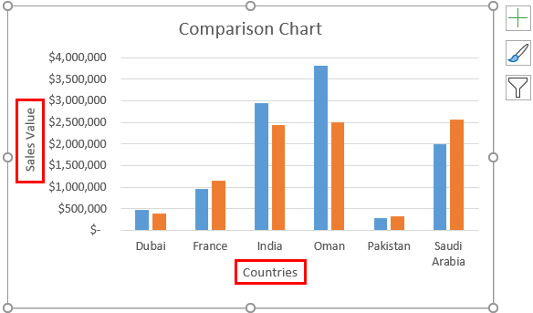
Comparison Chart in Excel | Adding Multiple Series Under Same Graph
How to add total labels to stacked column chart in Excel? 1. Create the stacked column chart. Select the source data, and click Insert > Insert Column or Bar Chart > Stacked Column. 2. Select the stacked column chart, and click Kutools > Charts > Chart Tools > Add Sum Labels to Chart. Then all total labels are added to every data point in the stacked column chart immediately.
7 Steps to make a professional looking column graph in Excel or PowerPoint | Think Outside The Slide
How to add data labels from different column in an Excel chart? Right click the data series in the chart, and select Add Data Labels > Add Data Labels from the context menu to add data labels. 2. Click any data label to select all data labels, and then click the specified data label to select it only in the chart. 3.

Waterfall Chart - Page 2 of 2 - Beat Excel!
How to Use Cell Values for Excel Chart Labels Select range A1:B6 and click Insert > Insert Column or Bar Chart > Clustered Column. The column chart will appear. We want to add data labels to show the change in value for each product compared to last month. Select the chart, choose the "Chart Elements" option, click the "Data Labels" arrow, and then "More Options."
Excel multi color column charts « projectwoman.com
Text Labels on a Vertical Column Chart in Excel - Peltier Tech Right click on the new series, choose "Change Chart Type" ("Chart Type" in 2003), and select the clustered bar style. There are no Rating labels because there is no secondary vertical axis, so we have to add this axis by hand. On the Excel 2007 Chart Tools > Layout tab, click Axes, then Secondary Horizontal Axis, then Show Left to Right Axis.
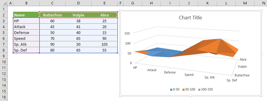
Surface Chart in Excel
Change axis labels in a chart - support.microsoft.com Right-click the category labels you want to change, and click Select Data. In the Horizontal (Category) Axis Labels box, click Edit. In the Axis label range box, enter the labels you want to use, separated by commas. For example, type Quarter 1,Quarter 2,Quarter 3,Quarter 4. Change the format of text and numbers in labels
Post a Comment for "41 excel column chart labels"